Poisson simulation

For the poisson background estimation problem, poisson.py, we explore different options for estimating the rate parameter \(\lambda\) from an observed number of counts. This program uses a Monte Carlo method to generate the true probability distribution \(P(\lambda)\) of the observed number of counts \(k\) coming from an underly rate \(\lambda\). We do this by running a Poisson generator to draw thousands of samples of \(k\) from each of a range of values \(\lambda\). By counting the number of times \(k\) occurs in each \(\lambda\) bin, and normalizing by the bin size and by the total number of times that \(k\) occurs across all bins, the resulting vector is a histogram of the \(\lambda\) probability distribution.

With this histogram we can compute the expected value as:

\[\hat\lambda = \int_0^\infty \lambda P(\lambda|k) d\lambda\]

and the variance as:

\[d\hat\lambda^2 = \int_0^\infty (\lambda - \hat\lambda)^2 P(\lambda|k) d\lambda\]

from __future__ import division, print_function
import numpy as np
from pylab import *

Generate a bunch of samples from different underlying rate parameters L in the range 0 to 20

P = np.random.poisson
L = linspace(0, 20, 1000)
X = P(L, size=(10000, len(L)))

Generate the distributions

P = dict((k, sum(X == k, axis=0)/sum(X == k)) for k in range(4))

Show the expected value of L for each observed value k

print("Expected value of L for a given observed k")
for k,Pi in sorted(P.items()):
    print(k, sum(L*Pi))

Show the variance. Note that we are using \(\hat\lambda = k+1\) as observed from the expected value table. This is not strictly correct since we have lost a degree of freedom by using \(\hat\lambda\) estimated from the data, but good enough for an approximate value of the variance.

print("Variance of L for a given observed k")
for k, Pi in sorted(P.items()):
    print(k, sum((L-(k+1))**2*Pi))

Plot the distribution of \(\lambda\) that give rise to each observed value \(k\).

for k, Pi in sorted(P.items()):
    plot(L, Pi/(L[1]-L[0]), label="k=%d"%k)
xlabel(r'$\lambda$')
ylabel(r'$P(\lambda|k)$')
xticks([0, 1, 2, 3, 4, 5, 6, 7, 8, 9, 10])
axis([0, 10, 0, 0.5])
title('Probability of underlying rate :math:`\lambda` for different observed $k$')
legend()
grid(True)
show()

Output:

Expected value of L for a given observed k
0 0.989473184121
1 2.00279003084
2 2.99802515025
3 3.9990621889
Variance of L for a given observed k
0 0.998074244206
1 2.00796671097
2 2.99095589399
3 3.99952301552

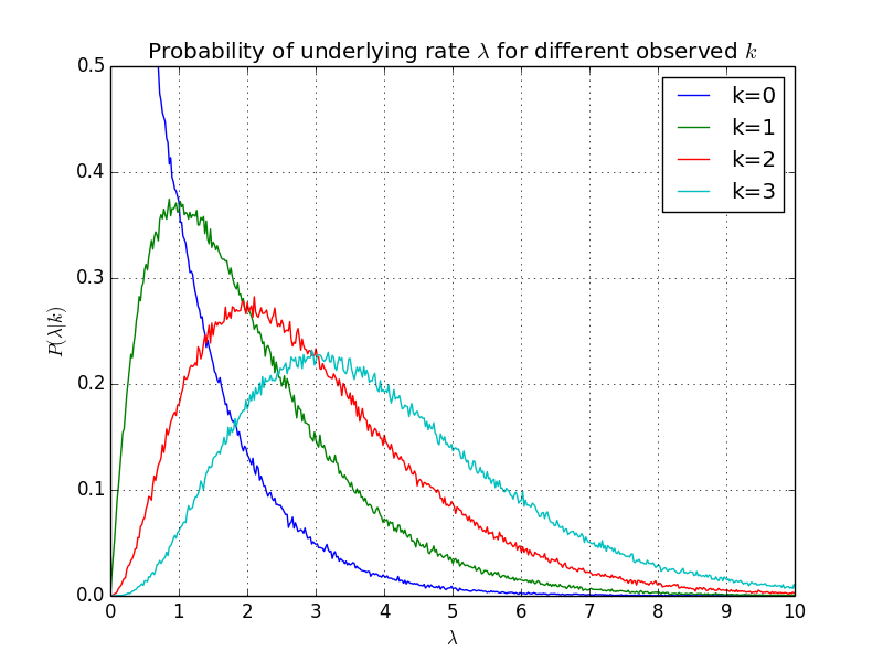
The figure clearly shows that the maximum likelihood value for \(\lambda\) is equal to the observed counts \(k\). Because the histogram is skew right, the expected value is a little larger, with an estimated value of \(k+1\), as seen from the output.

Download: sim.py.