Fitting a curve

Fitting a curve to a data set and getting uncertainties on the parameters was the main reason that bumps was created, so it should be very easy to do. Let’s see if it is.

First let’s import the standard names:

from bumps.names import *

Next we need some data. The x values represent the independent variable, and the y values represent the value measured for condition x. In this case x is 1-D, but it could be a sequence of tuples instead. We also need the uncertainty on each measurement if we want to get a meaningful uncertainty on the fitted parameters.

x = [1, 2, 3, 4, 5, 6]
y = [2.1, 4.0, 6.3, 8.03, 9.6, 11.9]
dy = [0.05, 0.05, 0.2, 0.05, 0.2, 0.2]

Instead of using lists we could have loaded the data from a three-column text file using:

data = np.loadtxt("data.txt").T
x, y, dy = data[0, :], data[1, :], data[2, :]

The variations are endless — cleaning the data so that it is in a fit state to model is often the hardest part in the analysis.

We now define the function we want to fit. The first argument to the function names the independent variable, and the remaining arguments are the fittable parameters. The parameter arguments can use a bare name, or they can use name=value to indicate the default value for each parameter. Our function defines a straight like of slope \(m\) with intercept \(b\) defaulting to 0.

def line(x, m, b=0):
    return m*x + b

We can build a curve fitting object from our function and our data. This assumes that the measurement uncertainty is normally distributed, with a 1-\(\sigma\) confidence interval dy for each point. We specify initial values for \(m\) and \(b\) when we define the model, and then constrain the fit to \(m \in [0, 4]\) # and \(b \in [-5, 5]\) with the parameter range method.

M = Curve(line, x, y, dy, m=2, b=2)
M.m.range(0, 4)
M.b.range(-5, 5)

Every model file ends with a problem definition including a list of all models and datasets which are to be fitted.

problem = FitProblem(M)

The complete model file curve.py looks as follows:

from bumps.names import *

x = [1, 2, 3, 4, 5, 6]
y = [2.1, 4.0, 6.3, 8.03, 9.6, 11.9]
dy = [0.05, 0.05, 0.2, 0.05, 0.2, 0.2]

def line(x, m, b=0):
    return m*x + b

M = Curve(line, x, y, dy, m=2, b=2)
M.m.range(0, 4)
M.b.range(-5, 5)

problem = FitProblem(M)

We can now load and run the fit:

$ bumps.py curve.py --fit=newton --steps=100 --store=T1

The --fit=newton option says to use the quasi-newton optimizer for not more than 100 steps. The --store=T1 option says to store the initial model, the fit results and any monitoring information in the directory T1.

As the fit progresses, we are shown an iteration number and a cost value. The cost value is approximately the normalized \(\chi^2_N\). The value in parentheses is like the uncertainty in \(\chi^2_N\), in that a 1-\(\sigma\) change in parameter values should increase \(\chi^2_N\) by that amount.

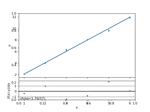
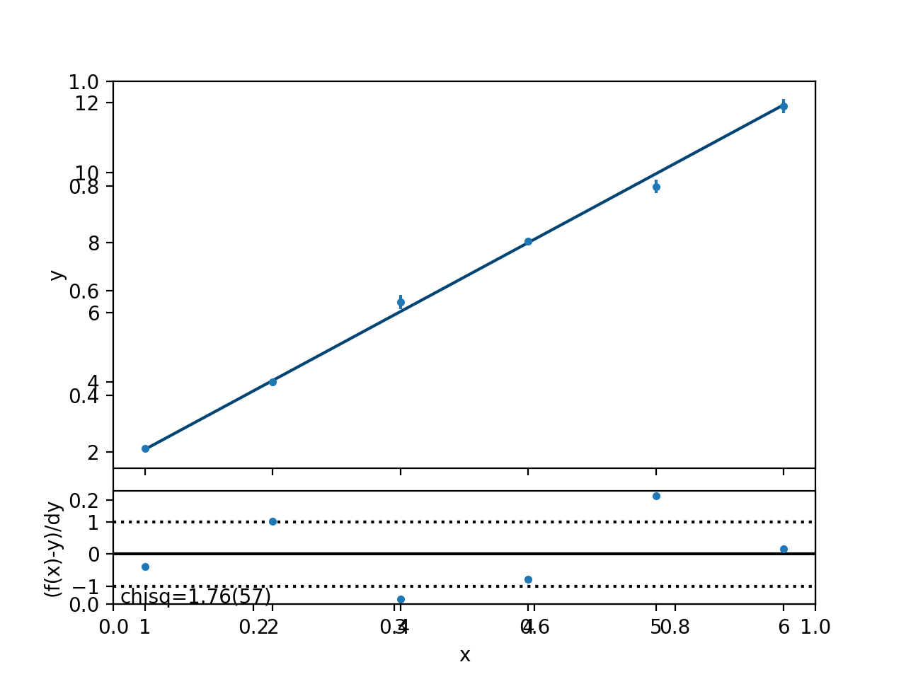
Here is the resulting fit:

(Source code, png, hires.png, pdf)

All is well: Normalized \(\chi^2_N\) is close to 1 and the line goes nicely through the data.

Download: curve.py.